NIST released its first version of PCASYS to the public in 1995. The two main changes in this new distribution are the addition of the multi-layer perceptron(MLP) classifier and replacing EISPACK routines with more stable CLAPACK routines[47] for computing eigen values and eigen vectors. Section 4.1.3.2 discusses the details of the MLP classifier. The CLAPACK routines have proven more stable and reliable across different operating systems. A large portion of the code has also been modified to be more general with the parameters of the input data. For example, the original version required fingerprints to be at least 512 *480 pixels, six output-classes in the classifier, and a 28 *30 array of ridge directions. The new code allows for variations in these sizes. While most of the code is more general, the core detection algorithm still requires a 32 *32 array of ridge directions and several parameters are tuned based on the old fixed dimensions that were used. For this reason many of the oldS,hardcodedT^ dimensions are still used, but they are defined in include files that the user could easily change and then retune other parameters as needed.
An adjustment was also made to the enhancement/ridge flow detection. Previously, the enhancement algorithm did local enhancement over the image every 24 *24 pixels, starting at a preset location(neartop-leftofimage). Similarly, the ridge flow algorithm used 16 *16 pixel averages starting at a different preset location. The enhancement has been adjusted to work on 16*16 pixel windows that are aligned with the window used in ridge flow averaging. This helps minimize the effect of enhancement artifacts whencomputingridgeflowaverages,whichoccur on the borders of the 16 *16 window, causing erroneous ridge flowpoints in the final orientation array. Interpolation was added to the final segmentation process but there was no improvement in the overall system performance, just an increase in preprocessing time. The old method of rounding to the nearest pixel was kept when doing segmentation. The interpolation routine is included in the sourcecode( sgmnt.c) but not used.
Finally, given the changes that were made to the feature extraction process, the parameters for the PNN classifier, mainly the regional weights and overall smoothing factor, were optimized to the new feature set.
This section describes the details of feature extraction and classification foreach fingerprint. Sections 4.1.1.1 and 4.1.1.2 are preprocessing steps to prepare the fingerprint image for feature extraction covered in Sections 4.1.1.3-4.1.1.5. Sections 4.1.1.6-0 discuss details of the neural network classifiers. Figure6 is an example print of the whorl class and will be used for subsequent figures illustrating the stages of processing.
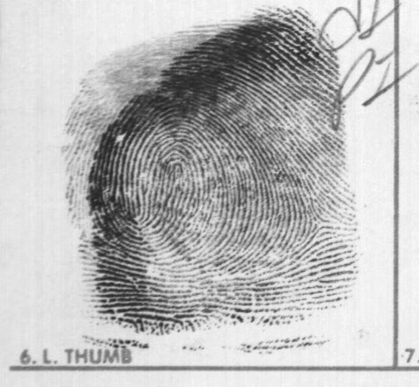
Figure 6. Fingerprint used to demonstrate the fingerprint classification process ( s0025236.wsq).
The segmentor routine performs the first stage of processing needed by the classifier. It reads the input fingerprint image. The image must be an 8-bit grayscale raster of width at least 512 pixels and height at least 480 pixels(these dimensions can be changed in the file include/pca.h), and scanned at about 19.69 pixels per millimeter(500 pixels per inch). The segmentor produces, as its output, an image that is 512 *480 pixels in size by cutting a rectangular region of these dimensions out of the inputimage. The sides of the rectangle that is cut out are not necessarily parallel to the corresponding sides of the original image. The segmentor attempts to position its cut rectangle on the impression made by the first joint of the finger. It also attempts to define the rotation angle of the cut rectangle and remove any rotation that the finger impression had to start with.
Cutting out this smaller rectangle is helpful because it reduces the amount of data that has to under go subsequent processing(especially the compute- intensive image enhancement). Removing rotation may help since it removes a source of variation between prints of the same class.2 2The images produced by the segmentor are similar to those of NIST Special Database 4 in which the corrections for translation and rotation were done manually.
(1) (2) (3) (4) (5) (6) (7)
Figure 7. Steps in the fingerprint segmentation process.
The segmentor decides which rectangular region of the image to snip out by performing a sequence of processing steps. This and all subsequent processing will be illustrated using the fingerprint from Figure6 as an example. Figure7 shows the results of the segmentorS^s processing steps.
First, the segmentor produces a small binary(two-valued or logical-valued) image. The binary image pixels indicate which 8 *8 -pixel blocks of the original image should be considered the foreground. Foreground is the part of the image that contains ink, whether from the finger impression itself or from printing or writing on the card. To produce this foreground-image, it first finds the minimum pixelvalue for each block and the global minimum and maximum pixel values in the image. Then, foreach of a fixed set of factor values between 0 and 1, the routine produces a candidate foreground-image based on factor as follows:
threshold = global_min + factor * (global_max - global_min) Set to true each pixel of candidate foreground-image whose corresponding pixel of the array of block minimais!threshold, and count resulting true pixels.
Count the transitions between true and false pixels in the candidate foreground-image, counting along all rows and columns. Keep track of the minimum, across candidate foreground-images, of the number of transitions. Among those candidate foreground-images whose number of true pixels is within predefined limits, pick the one with the fewest transitions. If threshold is too low, there tend to be many white holes in what should be solid blocks of black foreground; if threshold is too high, there tend to be many black spots on what should be solid white background. If threshold is about right, there are few holes and few spots, hence few transitions. The first frame in Figure7 shows the resulting foreground-image.
Next, the routine performs some cleanup work on the foreground-image, the main purpose of which is to delete those parts of the foreground that correspond to printing or writing rather than the finger impression. The routine does three iterations of erosion 3 then deletes every connected set of true pixels except the one whose number of true pixels is largest. The final cleanup step sets to true, in each row, every pixel between the left most and rightmost true pixels in that row, and similarly for columns. The routine then computes the centroid of the cleaned-up foreground- image, for later use. These condframe in Figure7 shows the result of this cleanup processing. Next, the routine finds the left, top and right edges of the foreground, which usually has a roughly rectangular shape. Because the preceding cleanup work has removed noise true pixels caused by printed box lines or writing, the following very simple algorithm is sufficient for 3 Erosion consists of changing to false each true pixel that is next to a false pixel. finding the edges. Starting at the middle row of the foreground-image and moving upward, the routine finds the leftmost true pixel of each row and uses the resulting pixels to trace the left edge. To avoid going around the corner onto the topedge, the routine stops when it encounters a row whose leftmost true pixel has a horizontal distance of more than 1 from the leftmost true pixel of the preceding row. The routine finds the bottompart of the left edge by using the same process but moving downward from the middlerow; and it finds the top and right edges similarly. The third, fourth, and fifth frames in Figure7 depict these edges. Next, the routine uses the edges to calculate the overall slope of the foreground.
First, it fits a straight line to each edge by linear regression. The left and right edges, which are expected to be roughly vertical, use lines of the form x=my+b and the top edge use the form y=mx+b. The next to last frame in Figure7 shows the fitted lines. The overall slope is defined to be the average of the slopes of the left-edge line, the right-edge line, and a line perpendicular to the top-edge line.
Having measured the foreground slope, the segmentor now knows the angle to which it should rotate its cutting rectangle to nullify the existing rotation of the fingerprint; but it still must decide the location at which to cut. To decide this, it first finds the foreground top, in a manner more robust than the original finding of the top edge and resulting fitted line. It finds the top by considering a tall rectangle, whose width corresponds to the output image width, whose center is at the previously computed centroid of the foreground-image, and is tilted in accordance with the overall foreground slope. Starting at the top row of the rectangle and moving downward, the routine counts the true pixels of each row. It stops at the first row which both fits entirely on the foreground-image and has at least a threshold number of true pixels. The routine then finishes deciding where to cut by letting the top edge of the rectangle correspond to the foreground top it has just detected. The cut out image will be tilted to cancel out the existing rotation of the fingerprint, and positioned to hang from the top of the foreground.
The last frame in Figure7 is the (cleaned-up) foreground with an outline super imposed on it showing where the segmentor has decided to cut. The segmentor finishes by actually cutting out the corresponding piece of the inputimage; Figure8 shows the resulting segmented image. (The routine also cuts out the corresponding piece of the foreground-image, for use later by the pseudo-ridge analyzer.)
Figure 8. The sample fingerprint after segmentation.
This step enhances the segmented fingerprint image. The algorithm used is basically the same as the enhance-merit algorithm described in[38], and pp.2-8-2-16 of [39] provide a description of other research that independently produced this same algorithm. The routine goes through the image and snips out a sequence of squares each of size 32 *32 pixels, with the snipping positions spaced 16 pixels apart in each dimension to produce overlapping. Each inputsquare under goes a process that produces an enhanced version of its middle 16 *16 pixels, and this smaller square is installed into the output image in a non-over lapping fashion relative to other output squares. (The overlapping of the input squares reduces boundary artifacts in the output image.)
The enhancement of an input square is done by first performing the forward two-dimensional fast Fourier transform(FFT) to convert the data from its original(spatial) representation to a frequency representation. Next, a nonlinear function is applied that tends to increase the power of useful information(the overall pattern, and in particular the orientation, of the ridges and valleys) relative to noise. Finally, the backward 2-dFFT is done to return the enhanced data to a spatial representation before snipping out the middle 16 *16 pixels and installing them into the output image. The filter's processing of a square of inputpixels can be described by the following equations. First, produce the complex-valued matrix A+iB by loading the square of pixels into A and letting B be zero. Then, perform the forward 2-d discrete Fourier transform, producing the matrix X+iY defined by
( ) ( )\Delta \Delta = = \Delta \Theta \Lambda \Xi \Pi \Sigma +-+=+ 31 0 31 0 32 2exp m n mnmnjkjk nkmj iiBAiYX \Phi
Change to zero a fixed subset of the Fourier transform elements corresponding to low and high frequency bands which, as discussed below, can be considered to be noise. Then take the power spectrum elements Xjk+Y jk of the Fourier transform, raise them to the 0.3 power, and multiply them by the Fourier transform elements, producing a new frequency-domain representation U+ iV: ( )
( )jkjkjkjkjkjk iYXYXiVU ++=+ 3.022 Return to a spatial representation by taking the backward Fourier transform of U+iV, ( ) ( )\Delta \Delta = = \Delta \Theta \Lambda \Xi \Pi \Sigma ++=+ 31 0 31 0 32 2exp j k jkjkmnmn knjm iiVUiDC \Phi
then finish up as follows: find the maximum absolute value of the elements of C(the imaginary matrix D is zero), and cut out the middle 16 *16 pixels of C and install them in the output image, but first applying to the man affine transform that maps 0 to 128(a middle gray) and that causes the range to be as large as possible without exceeding the range of 8-bit pixels(0 through 255). The DC component of the Fourier transform is among the low-frequency elements that are zeroed out, so the mean of the elements of C is zero; there fore it is reasonable to map 0 to the middle of the available range. However, for greater efficiency, the enhancer routine actually does not simply implement these formulas directly. Instead, it uses fast Fourier transforms(FFTs), and takes advantage of the purely real nature of the input matrix by using 2-d real FFTs.
The output is no different than if the above formulas had been translated straight into code. We have found that enhancing the segmented image with this algorithm, before extracting the orientation features, increases the accuracy of the resulting classifier. The table and graphs on pp.24-6 of[24] show the accuracy improvement caused by using this filter(localized FFT filter), as well as the improvements caused by various other features. The nonlinear function applied to the frequency-domain representation of the square of pixels has the effect of increasing the relative strength of those frequencies that were already dominant. The dominant frequencies correspond to the ridges and valleys in most cases. So the enhancer strengthens the important aspects of the image at the expense of noise such as small details of the ridges, breaks in the ridges, and inkspots in the valleys. This is not simply a linear filter that attenuates certain frequencies, although part of its processing does consist of eliminating low and high frequencies. The remaining frequencies go through a nonlinear function that adapts to variations as to which frequencies are most dominant. This aspect of the filter is helpful because the ridge wavelength can vary considerably between fingerprints and between areas within a single fingerprint. 4 Figure9 shows the enhanced version of the segmented image. At first glance, a noticeable difference seen between the original and enhanced versions is the increase in contrast. The more important change caused by the enhancer is the improved smoothness and stronger ridge/valley structure of the image, which are apparent upon closer examination. Discontinuities are visible at the boundaries of some output squares despite the overlapping of input squares, but these apparently have no major harmful effect on subsequent processing, due to alignment of the enhanced tiles with the orientation detection tiles. 4
A different FFT-based enhancement method, the directional FFT filter of [24], uses global rather than local FFTs and uses a set of masks to selectively enhance regions of the image that have various ridge orientations. This enhancer was more computationally intensive than the localized FFT filter, and did not produce better classification accuracy than the localized filter.
Figure 9. Sample fingerprint after enhancement.
This step detects, at each pixel location of the fingerprint image, the local orientation of the ridges and valleys of the finger surface, and produces an array of regional averages of these orientations. This is the basic feature extractor of the classification.
Figure 10. Pattern of slits (i = 1-8) used by the orientation detector.
The routine is based on the ridge-valley fingerprint binarizer described in[40]. That binarizer uses the following algorithm to reduce a grayscale fingerprint image to a binary(black and white only)image. For each pixel of the image, denoted C in Figure10, the binarizer computes slit sums s i,i=1...8,where each si,is the sum of the values of the slit of four pixels labeled i(i.e.,1-8)in the figure. The binarizer uses local thresholding and slit comparison formulas. The local thresholding formula sets the output pixel to white if the value of the central pixel, C, exceeds the average of the pixels of all slits, that is, if
\Delta => 8 132 1 i isC (1) 7 8 1 2 3 6 7 8 1 2 3 46 4 5 5 C 5 54 6 4 3 2 1 8 7 6 3 2 1 8 7
Local thresholding such as this is better than using a single threshold every where on the image, since it ignores gradual variations in the overall brightness. The slit comparison formula sets the output pixel to white if the average of the minimum and maximum slit sums exceeds the average of all the slit sums, that is, if
( ) \Delta =>+ 8 1 maxmin 8121 i isss (2)
The motivation for this formula is as follows. If a pixel is in a valley, then one of its eight slits will lie along the (light) valley and have a high sum. The other seven slits will each cross ridges and valleys and have roughly equal lower sums. The average of the two extreme slit sums will exceed the average of all eight slit sums and the pixel will be binarized correctly to white. Similarly, the formula causes a pixel lying on a ridge to be binarized correctly to black. This formula uses the slits to detect long structures(ridges and valleys), rather than merely using their constituent pixels as a sampling of local pixels as formula1 does. It is able to ignore small ridge gaps and valley blockages, since it concerns itself only with entire slits and not with the value of the central pixel. The authors of[40] found that they obtained good binarization results by using the following compromise formula, rather than using either(1) or (2) alone: the output pixel is set to white if
\Delta =>++ 8 1maxmin 8 34
i isssC (3) This is simply a weighted average of (1) and (2), with the first one getting twice as much weight as the second.
This binarizer can be converted into a detector of the ridge or valley orientation at each pixel. A pixel that would have been binarized to black(a ridge pixel) gets the orientation of its minimum- sum slit, and a pixel that would have been binarized to white(a valley pixel)gets the orientation of its maximum-sum slit. However,the resulting array of pixel-wise orientations is large, noisy, and coarsely quantized(only 8 different orientations are allowed). There fore, the pixel-wise orientations are reduced to a much smaller array of local average orientations, each of which is made from a 16OE16 square of pixel-wise orientations. The averaging process reduces the volume of data, decreases noise, and produces a finer quantization of orientations.
The ridge angle "is defined to be 0 r^if the ridges are horizontal and increasing towards 180 oas the ridges rotate counter clockwise(0 o=!"!180o). When pixel-wise orientations are averaged, the quantities averaged are not actually the pixel-wise ridge angles ",but rather the pixel-wise orientation vectors (cos2",sin2 "). The orientation finder produces an array of these averages of pixel-wise orientation vectors.
5Since all pixel-wise vectors have length 1(being cosine, sine pairs), each average vector has a length of at most 1. If a square of the image does not have a well-defined overall ridge and valley orientation, then the orientation vectors of its 256 pixels will tend to cancel each other out and produce a short average vector. This can occur because of 5 Averaging a set of local orientation angles can produce absurd results, because of the non-removable point of discontinuity that is inherent in an angular representation, so it is better to use the vector representation. Also, the resulting local average orientation vectors are anappropriate representation to use for later processing, because these later steps require that Euclidean distances between entire arrays of local average orientations produce reasonable results.
Note:The R92 registration program requires converting the vectors into angles of a different format. blurring or because the orientation is highly variable within the square. The length of an average vector is thus a measure of orientation strength. The routine also produces as output the array of pixel-wise orientation indices, to be used by a later routine that produces a more finely spaced array of average orientations. Figure11 depicts the local average orientations that were detected in the segmented and filtered image from the example fingerprint.
Figure 11. Array of local average orientations of the example fingerprint Each bar, depicting an orientation, is approximately parallel to the local ridges and valleys.
Registration is a process that the classifier uses in order to reduce the amount of translation variation between similar orientation arrays. If the arrays from two fingerprints are similar except for translation, the feature vectors that later processing steps will produce from these orientation arrays maybe very different because of the translation. This problem can be improved by registering each array(finding a consistent feature and essentially translating the array, bringing that feature to standard location).
To find the consistent feature that is required, we use the R92 algorithm of Wegstein[8]. The R92 algorithm finds, in an array of ridge angles, a feature that is used to register the fingerprint. The feature R92 detects in a loop and whorl fingerprint is located approximately at the core of the fingerprint. The algorithmal so finds a well-defined feature in arch and tented arch fingerprints although these types of prints do not have true cores. After R92 finds this feature, which will be denoted the registration point, registration is completed by taking the array of pixel-wise orientations produced earlier and averaging 16 *16 squares from it to make a new array of average orientations. The averaging is done the same way it was done to make the first array of average orientations (which became the input to R92). In addition, the squares upon which averaging is performed are translated by the vector that is the registration point minus a standard registration point defined as the component-wise median of the registration points of a sample of fingerprints. The result is a registered array of average orientations.6 The R92 algorithm begins by analyzing the matrix of angles in order to build the S,K-table.T^R92 processes the orientations in angular form. It defines angle ranges from 0 r^ to 90r^ as a ridge rotates from horizontal counter clockwise to vertical, and 0 r^ to U""90 r^ for clockwise rotation. These angles differ from the earlier range 0 r^ to 180r^ as the ridge rotates counterclockwise from horizontal. This table lists the first location in each row of the matrix where the ridge orientation changes from positive slope to negative slope to produce a well-formed arch. Associated with each K-table entry are other elements that are used later to calculate the registration point. The ROW and COL values are the position of the entry in the orientation matrix. The SCORE is how well the arch is formed at this location. The BCSUM is the sum of this angle with its east neighbor, while the ADSUM is BCSUM plus the one angle to the west and east of the BCSUM. SUM HIGH and SUMLOW are summations of groups of angles below the one being analyzed. For these two values, five sets of four angles are individually summed, and the lowest and highest are saved in the K-table.
With the K-table filled in, each entry is then scored. The score indicates how well the arch is formed at this point. The point closest to the core of the fingerprint is intended to get the largest score. If scores are equal, the entry closest to the bottom of the image is considered the winner. Calculating a score for a K-table entry uses six angles and one parameter, RK3. RK3 is the minimum value of the difference of two angles. For this work, the parameter was set at 0 degrees, which is a horizontal line. The six angles are the entry in the K-table, the two angles to its left and the three angles to its right. So if the entry in the K-table is( i,j), then the angles are at positions(i,j-2), (i,j-1), (i,j), (i,j+1), (i,j+2), and(i,j+3). These are labeled M,A,B,C,D, and N, respectively. For each of the differences, M-B,A - B,C-N ,and C-D ,greater than RK3, the score is increased by one point. If A has a positive slope, meaning the angle of A is greater than RK3, or if M-A is greater than RK3, the score is increased by one point. If D has a negative slope, meaning the angle of D is less than RK3, or if D-N is greater than RK3, then the score is increased by one point. If N has a negative slope, then the score is increased by one point. All these comparisons form the score for the entry.
Using the information gathered about the winning entry, a registration point is produced. First, it is determined whether the fingerprint is possibly an arch; if so, the registration point( x, y) is computed as:
( )( ) ( ) \Omega ff + \Delta \Delta \Theta \Lambda \Xi \Xi \Pi \Sigma -+ +-= 11,, , C CRACRA CRAx ( ) ( ) ( )( ) ( ) ( )( ) ( )( ) ( ) ( ) 11 1211 -+++ -+-++-+++= ktsktskts ktsRktsRktsRy \Omega ff\Omega ff\Omega ff
where A is the angle at an entry position, R is the row of the entry, C is the column of the entry, k is the entry number, ts is a sum of angles,!is 16(the number of pixels between orientationloci), 6 The new array is made by re-averaging the pixel-wise orientations with translated squares, rather than just translating the first average-orientation array. This is done because the registration point found by R92, and hence the prescribed translation vector, is defined more precisely than the crude 16-pixel spacing corresponding to one step through the average orientation array. and "is 8.5. The ts value is calculated by summing up to six angles. These angles are the current angle and the five angles to its east. While the angle isnS^t greater than 99 o,its absolute value is added to ts.For angles89,85,81,75,100, and 60, the sum would be 330(89+85+81+75).Since 100 is greater than99, the summation stops at 75.
For an image that is possibly something other than an arch, the computation of the registration point is slightly more complex:
( ) ( )1,,1 +-= CRACRAdsp ( ) ( )1,1,12 ++-+= JLRAJLRAdsp \Delta \Theta \Lambda >== otherwisedsp dspdh 901 9011 ff ff ( ) \Delta \Theta \Lambda >-= otherwise dspdspdh 0 902909022 ff ( ) 221 dhdhdh += ( )( ) ( ) \Omega ff + \Delta \Delta \Theta \Lambda \Xi \Xi \Pi \Sigma -+ +-*= 11,, ,1 C CRACRA CRAxx ( ) \Omega ff +\Delta \Delta \Theta \Lambda \Xi \Xi \Pi \Sigma -++= 1 2 ,12 JL dsp JLRAxx ( ) 221 xx ds xxxxdhx +-=
dhRy -= ff Where A,R,C,ff, and \Omega areas before and JL is the cross-reference point column. The left picture in Figure12 shows the orientation array of the example fingerprint with its registrationpoint, and the standard registration point is marked; the right picture shows the resulting registered version of the orientation array. Obviously some lower and left areas of the registered array are devoid of data, which would have had to be shifted in from undefined regions. Likewise, data that were in upper and right areas have fallen off the picture and are lost; but the improved classification accuracy that we have obtained as a result of registration shows that this is no great cause for concern. The optimal pattern of regional weights, discussed later, also shows that outer regions of the orientation array are not very important. The test results in [24]show that registration improves subsequent classification accuracy.
Figure 12. Left: Orientation array Right: Registered orientation array. The plus sign is registration point (core) found by R92, and plus sign in square is standard (median) registration point.
This step applies a linear transform to the registered orientation array. Transformation accomplishes two useful processes. First, the reduction of the dimensionality of the feature vector from its original 1680 dimensions to 64 dimensions(PNN) and 128 dimensions(MLP). Second, the application of a fixed pattern of regional weights(PNNonly) which are larger in the important central area of the orientation array.
The size of the registered orientation array(oa) representing each fingerprint is1 680elements(28*30 orientation vectors OEtwo components per orientation vector). The size of these arrays makes it computationally impractical to use them as the feature inputs into either of the neuralnetwork classifiers(PNN/MLP).
It would be helpful to transform these high-dimensional feature vectors into much lower-dimensional ones in such a way that would not be detrimental to the classifiers. Fortunately, the Karhunen-Loe`ve(K-L)transform[41] does exactly that. To produce the matrix that implements the K-L transform, the first step is to make the sample covariance matrix of a set of typical original feature vectors, the registered orientation arrays in our case. Then, a routine is used to produce a set of eigen vectors of the covariancematrix, corresponding to the largest eigenvalues; let m denote the number of eigen vectors produced. Then, for any n ! m, the matrix w can be defined to have as its columns the first n eigen vectors; each eigen vector has as many elements as an original feature vector, 1680 in the case of orientation arrays. A version of aK-L transform 7, 7Usually the sample mean vector is subtracted from the original feature vector before applying !t, but we omit this step because doing so simplifies the computations and has no effect on the final results of either classifier.
If the user needs it, a full version, that subtracts the mean vector from each feature vector, is included in src/bin/kltran. which reduces an original feature vector u(an orientation array, thought of as a single 1680-dimensional vector)to a vector w of n elements, can then be defined as follows: u!w t= The K-L transform thus maybe used to reduce the orientation array of a fingerprint to a much lower-dimensional vector, which maybe sent to the classifier. This dimension reduction produces approximately the same classification results as would be obtained without the use of the K-L transform but with large savings in memory and compute time. A reasonable value of n, the number of eigen vectors used and hence number of elements in the feature vectors produced, can be found by trial and error; usually n can be much smaller than the original dimensionality. We have found 64 to be a reasonable n for PNN and 128 for MLP. In earlier versions of our fingerprint classifier, we produced low-dimensional feature vectors in this manner, using the arrays of (28OE30) orientation vectors as the original feature vectors.
However, later experiments revealed that significantly better classification accuracy could be obtained by modifying the production of the feature vector. The modification allows the important central region of the fingerprint to have more weight than the outer regions; what we call regional weights. This is discuss in the next section.
During testing, it was noted that the uniform spacing of the orientation measurements throughout the picture area could probably be improved by using a non-uniform spacing. The non-uniform spacing concentrated the measurements more closely together in the important central area of the picture and had a sparser distribution in the outer regions. We tried this [23], keeping the total number of orientation measurements the same as before(840) in order to make a fair comparison, and the result was indeed a significant lowering of the classification error rate.
Eventually, we realized that the improved results might not have been caused by the non-uniform spacing but rather by the mere assignment of greater weight to the central region, caused by placing a larger number of measurements there. We tested this hypothesis by reverting to the uniformly spaced array of orientation measurements, but now with a non-uniform pattern of regional weights applied to the orientation array before performing the K-L transform and computing distances. The application of a fixed pattern of weights to the features before computing distances between feature vectors is equivalent to the replacement of the usual Euclidean distance by an alternative distance . In [42], Specht improves the accuracy of PNN in about the same manner:pp.1-765-6 described the method used to produce a separate ffi value for each dimension(feature).
To keep the number of weights reasonably small and thus controlthe amount of runtime that would be needed to optimize them, we decided to assign a weight to each 2 *2 block of orientation-vectors. This produced 210(14 *15)weights, versus assigning a separate weight to each of the 840 orientation-vectors. Optimization of the weights was done using a very simple form of gradient descent, as discussed in Section 4.1.3.1.1. The resulting optimal(or nearly optimal) weights are depicted in Figure13. The graytones represent the absolute values of the weights(their signs have no effect), with the values mapped to tones by a linear mapping that maps 0 to black and the largest absolute value that occurred, to white. These weights canbe representedasa diagonal matrix W of order 1680. Their application to an original featurevector(orientation array)u, to produce a weighted version", is given by the matrix multiplication Wuu =~ We have tried optimizing a set of weights to be applied directly to the K-Lfeatures, but this produced poor generalization results. The regional weights described here are not equivalentto any set of weights (diagonal matrix) that could be applied to the K-L features. Their use is approximately equivalent to the application of the non-diagonal matrix fflfflfflffltWfflfflfflffl mentioned in Section 4.1.3.1.1, to the K-L feature vectors. We also have tried optimizing a completely unconstrained linear transform(matrix) to be applied to the K-L feature vectors before computing distances; that produced impressive lowering of the error during training but disastrous generalization results. Among our experiments involving the application of linear transforms prior to PNN distance computations, we obtained the best results by using regional weights.
Figure 13. Absolute values of the optimized regional weights. Each square represents one weight, associated with a 2 ****2 block from the registered orientation array.
Clearly, it is reasonable to apply the optimized regional weights W, and then to reduce dimensionality with fflfflfflfflt before letting the PNN classifier compute distances. An efficient way to do this is to make the combined transform matrix T=fflfflfflffltW then when running the classifier on a fingerprint, to use Tuw = to convert its orientation array directly into the final feature-vector representation.8
8Alter optimizing the weights W, we could have made new eigen vectors from the covariance matrix of the weighted original-feature vectors. The fflfflfflffltW resulting from this new fflfflfflfflt would presumably have then produced a more efficient dimensionality reduction than we now obtain, allowing the use of fewer features. We decided not to bother with this, since the memory and time requirements of the current feature vectors are reasonable.
This step takes as its input the low-dimensional feature vector that is the output of the transform discussed in Section 4.1.3.1, and it determines the class of the fingerprint. The Probabilistic NeuralNetwork(PNN) is described by Spechtin[43]. The algorithm classifies an incoming feature vector by computing the value, at its point in feature space, of spherical Gaussian kernel functions centered at each of a large number of stored prototype feature vectors. These prototypes were made ahead of time from a training set of fingerprints of known class by using the same preprocessing and feature extraction that was used to produce the incoming feature vector. For each class, an activation is made by adding up the values of the kernels centered at all prototypes of that class; the hypothesized class is then defined to be the one whose activation is largest. The activations are all positive, being sums of exponentials. Dividing each of the activations by the sum of all activations produces a vector of normalized activations, which, as Specht points out, can be used as estimates of the posterior probabilities of the several classes. In particular, the largest normalized activation, which is the estimated posterior probability of the hypothesized class, is a measure of the confidence that may be assigned to the classifier's decision.9 In mathematical terms, the above definition of PNN can be written as follows, starting with notational definitions:
N = number of classes(6inPCASYS)M

i = number of prototype prints of class i(1!i!N))(i

jx  = feature vector from jth prototype print of
classi(1!j!Mi)w = feature vector of the print to be classified

" = a smoothing factor a

i = activation for class ia~ i = normalized activation for
classih=hypothesized class

c=confidence Foreach classi, the PNN computes an activation:
( )( ) ( )( )( )\Delta = ---= iM j ijtijia 1 exp xwxw\Omega
It then defines h to be the i for which a i is greatest, and defines c to be the hth normalized activation:
\Delta === N i ihh aaac 1 ~
9 This naive version of PNN must compute the distance of the incoming feature vector from each of the many prototype feature vectors, possibly many cycles. Various methods have been found for increasing the speed of nearest-neighbors classifiers, a category PNN may be considered to fall into(see, for example ,[44], and [45] for a very fast tree method). The classification accuracy of fast approximations to the naive PNN may suffer at high rejection levels. For that reason, and because the naive PNN takes only a small fraction of the total time used by the PCASYS classification system(image enhancement takes much longer), we have used the naive version.
Figure14 is a bar graph of the normalized activations produced for the example fingerprint. Although PNN only needs to normalize one of the activations, namely the largest, to produce the confidence, all 6 normalized activations are shown here. The whorl(W) class has won and so is the hypothesized class(correctly as it turns out), but the left loop(L) class has also received a fairly large activation and therefore the confidence is only moderately high.
Figure 14. PNN output activations for the example fingerprint.
Figure 15. MLP output activations for the example fingerprint.
This alternative classifier takes as input the low-dimensional feature vector, non-optimized, as discussed in Sections 4.1.1.5 and 4.1.2.4 and a set of MLP weights. The weights are the result of several training runs of MLP in which the weights are optimized to produce the best results with the given training data. Section 4.1.3 discusses the training process in more detail. The output of mlp_single() is a set of confidence levels foreach of the possible output classes and an indication of which hypothetical class had the highest confidence. Figure15 shows the MLP output activations for the example fingerprint. The whorl(W) class has the highest activation and is the correct answer.
This step takes a grid of ridge orientations of the incoming fingerprint and traces pseudo-ridges [46], which are trajectories that approximately follow the flow of the ridges. By testing the pseudo-ridges for concave-upward shapes, the routine detects some whorl fingerprints that are misclassified by the classifiers. We were motivated to produce a whorl-detect or when we realized, upon examining the prints misclassified by the NN classifiers, that many of them were whorls.
The routine takes as input an array of local averaged ridge orientations. 10 Another input is a small binary image that shows the region of the segmented image comprising the inked foreground rather than the lighter background. First, the routine changes to zero vectors any of the orientation vectors that either are not on the foreground, or are smaller than a threshold in squared length. (Small squared length indicates uncertainty as to the orientation.) Next, it performs a few iterations of a smoothing algorithm, which merely replaces each vector by an average of itself and its four neighbors; this tends to improve anomalous or noisy vectors. Then, it finds out which vectors are either off the foreground or, in their now smoothed state, smaller than a threshold in squared length, and it marks these locations as bad, so that they will not be used later. The program also makes some new representations of the orientation vectors-as angles, and as step-vectors of specified length - which it uses later for efficient tracing of the pseudo-ridges(an implementation detail).
Having finished with this preliminary processing, the process then traces pseudo-ridges. Starting at a block of initial locations in the orientation array, it makes a pseudo-ridge by following the orientation flow, first in one of the two possible directions away from the initialpoint and then in the other direction. For example, if the ridge orientation at an initial point isS, northeast- southwestT^ then the program starts out in a northeast direction, and later comes back to the initial point and goes in a southwest direction. If a location has been marked as bad, then no trajectories are started there. A trajectory is stopped if it reaches a limit of the array of locations, reaches a bad location, if the turn required in the trajectory is excessively sharp, or if a specified maximum number of steps have been taken. The two trajectories traced out from an initial point are joined end to end, producing a finished pseudo-ridge. The pseudo-ridge only approximately follows the ridges and valleys, and is insensitive to details such as bifurcations or small scars. 10 The array used has its constituent orientation vectors spaced half as far apart as those comprising the arrays used earlier, and it does not undergo registration.
Figure 16. Left: Pseudo-ridges traced to find concave-upward lobe. Right: Concave-upward lobe that was found.
After the routine has finished tracing a pseudo-ridge, it goes through it from one end to the other and finds each maximal segment of turns that are either all left(or straight) turns, or all right turns. These segments can be thought of as lobes, each of which makes a sweep in a constant direction of curvature. A lobe qualifies as a concave upward shape, if itS^s orientation, at the sharpest point of curvature(vertex), is close to horizontal and concave upward, and it has a minimum amount of cumulative curvature on each side of itS^s vertex. The routine checks each lobe of the current pseudo-ridge to findout if the lobe qualifies as a concave upward shape. If no lobe qualifies, it advances to the next location in the block of initial points and makes a new pseudo-ridge. The routine stops when it either finds a concave upward shape or exhausts all lobe so fall pseudo-ridges without finding one. The final output shows if it did or did not find a concave upward shape. Figure16 shows a concave upward shaped lobe that was found. This pseudo-ridge tracer is useful as a detector of whorls. It rarely produces a false positive, defined as finding a concave upward lobe in a print that is not a whorl. It is more likely to produce a false negative, defined as not finding a concave upward lobe although a print is a whorl. The next section describes a simple rule that is used to combine the pseudo-ridge tracer's output with the output of the main classifier(PNN or MLP), there by producing a hybrid classifier that is more accurate than the main classifier alone.
The ridge tracer has many parameters that may be experimented with if desired as well as the parameter for combining the classifier and ridge tracing results(Section0), but reasonable values are provided in the default parameter file.
This final processing module takes the outputs of the main NeuralNetwork(NN) classifier and the auxiliary pseudo-ridge tracer, and makes the decision as to what class, and confidence, to assign to the fingerprint.
The NN classifier produces a hypothesized class and a confidence. The pseudo-ridge tracer produces a single bit of output, whose two possible values can be interpreted as the print is a whorl and it is not sure whether the print is a whorl. The pseudo-ridge tracer is never sure that a print is not a whorl. A simple rule was found for combining the NN and pseudo-ridge tracer results, to produce a classifier more accurate than the NN alone. The rule is described by this pseudo-code:
if(pseudo-ridge tracer says whorl) { hypothesized-class = whorl if(pnn_hypothesized_class == whorl) confidence = 1. else confidence = .9 } else { /* pseudo-ridge tracer says not clear whether whorl */ hypothesized_class = pnn_hypothesized_class confidence = pnn_confidence }
This is a reasonable way to use the pseudo-ridge tracer as a whorl detector, because as noted in the preceding section, this detector has very few false positives but a fair number of false negatives. So, if the whorl detector detects a whorl, the print is classified as a whorl even if the NN disagrees, although disagreement results in slightly lower confidence, since whorl detection implies that the print is almost certainly a whorl. If the whorl detector does not detect a whorl, then the NN sets the classification and confidence.
Since the whorl detector detected a whorl for the example print and the NN classified this print as a whorl, the final output of the classifier had a hypothesized class of whorl and a confidence of 1. As it turns out, this is the best possible result that could have been obtained for this print, since it actually is a whorl.
The pseudo-ridge tracer improves the result for someprints the NN would have correctly classified as whorls anyway(such as the example print), by increasing the classification confidences. It also improves the result for some whorls that the NN misclassifies, by causing them to be correctly classified as whorls. The tracer harms the result only for a very small number of prints, the non-whorls that it mistakenly detects to be whorls. The overall effect of combining the pseudo-ridge tracer with the main NN classifier is a lowering of the error rate, compared to the rate obtained using the NN alone.